Classification and Regression Tree (CART) Analysis Results Help Page
More information on how to start an analysis can be found in our CART Analysis Guide
Steps to View Results:
-
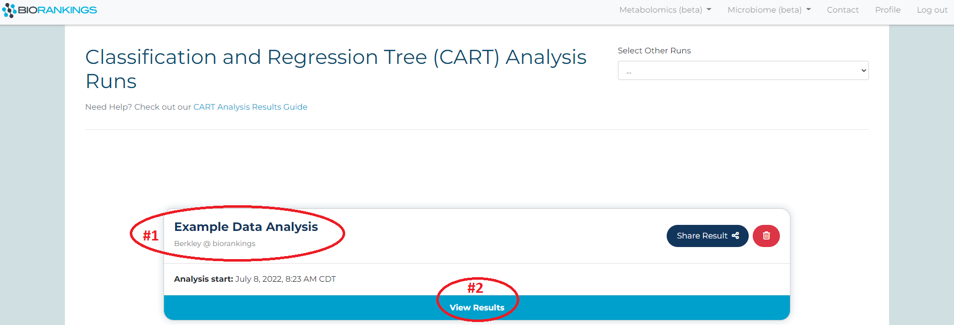
Once an analysis is complete it will appear on the
results page.
Click ‘View Result’ for more options and to view more information on that result. Below the test
name used from the demo data is shown with a red #1 and the 'View Result' is shown with a red #2.
-
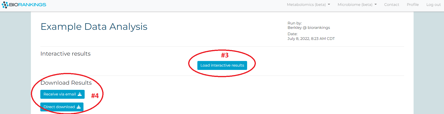
Click on ‘Load interactive results’ to load the interactive results page (red #3). Your interactive
results page will then begin loading and may take a few minutes. The ‘Get results’ button (red #4) will
send an email with the .pdf and .csv result files.
-
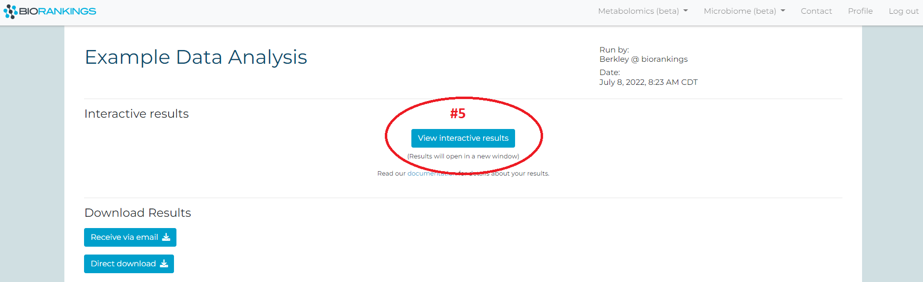
You will see a button labeled ‘View interactive results’ (red #5) once the loading process is
complete. Click the button and a new tab will pop up with your interactive results.
-
The interactive results page is available for 3 hours. You can always re-open a new
interactive window by going back to the result page and re-clicking ‘Load interactive
results’.
What do the results mean?
-
Below is the interactive results page.
-
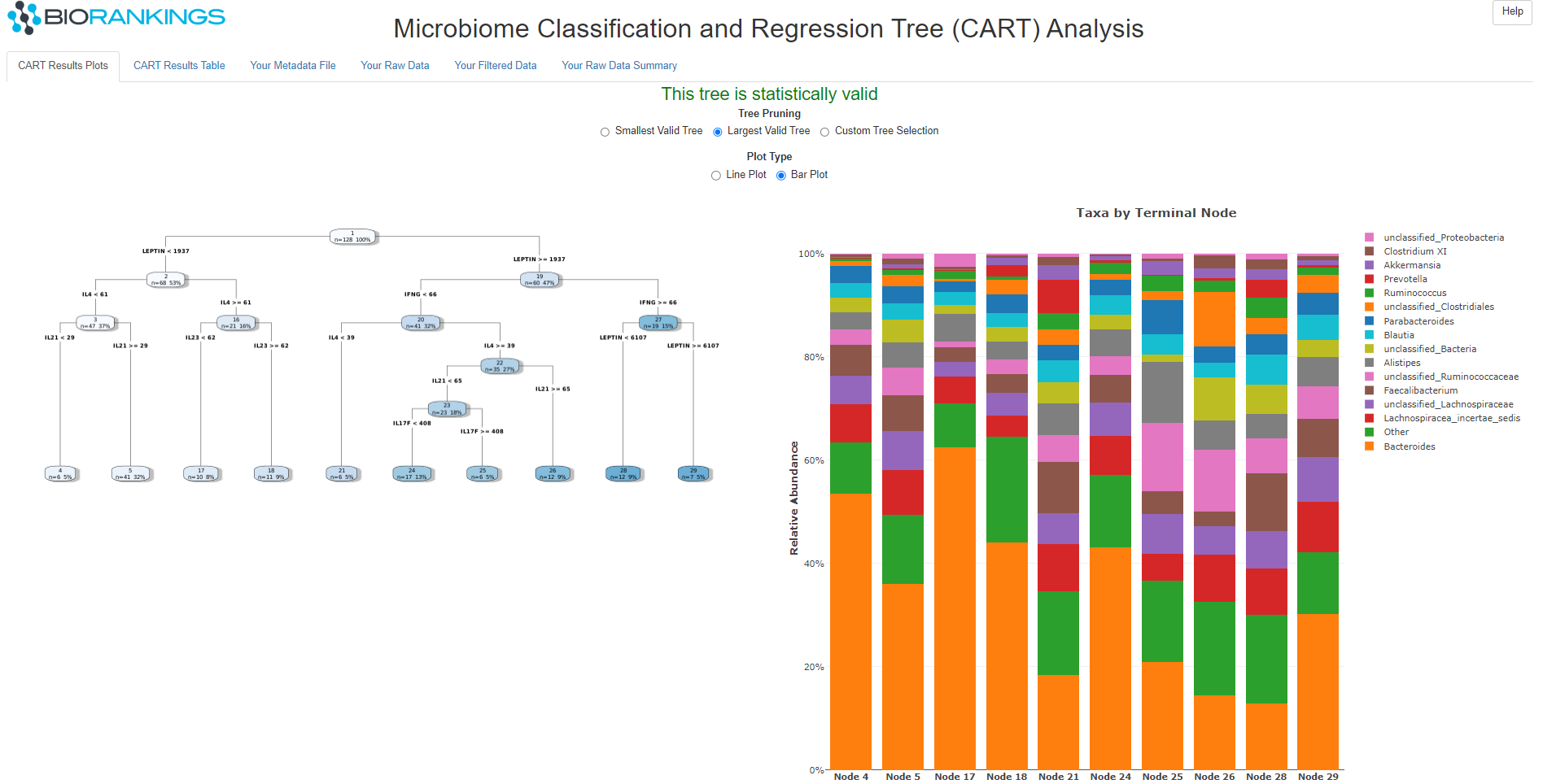
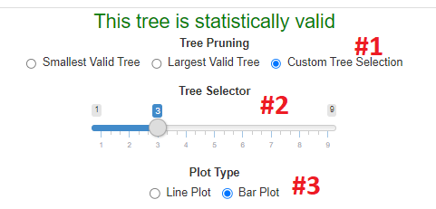
The first thing to note is the tree pruning selector. This allows the user to select the smallest,
the largest or a custom size tree (red #1). When the custom option is selected a slider bar will
appear (red #2). In the example below, the 3rd tree is selected on the custom slider bar.
There is also an option to switch the taxa abundance plot between a line plot and a bar plot (red #3).
Note: Not every tree selected via the custom option will be statistically valid.
-
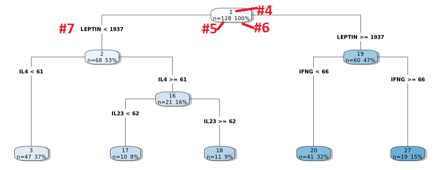
The classification tree consists of nodes and edges. Each node has a node number at the top
of the bubble (red #4), the number of samples in that node (red #5) and the percentage of the data
those samples make up (red #6). The edges show the covariate spliting rules (red# 7). In the example below the
1st node is split on LEPTIN, with node 2 containing samples with LEPTIN < 1937 and node 19 containing
samples with LEPTIN >= 1937.
-
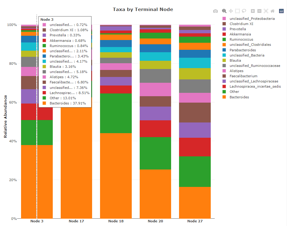
The final plot (either line or bar) shows the break down of taxa by the terminal nodes (a 'PI' plot). In the
example below, there are 5 terminal nodes (labeled Node 3, 17, 18, 20, 27) that match the
terminal node numbers in the tree plot.
-
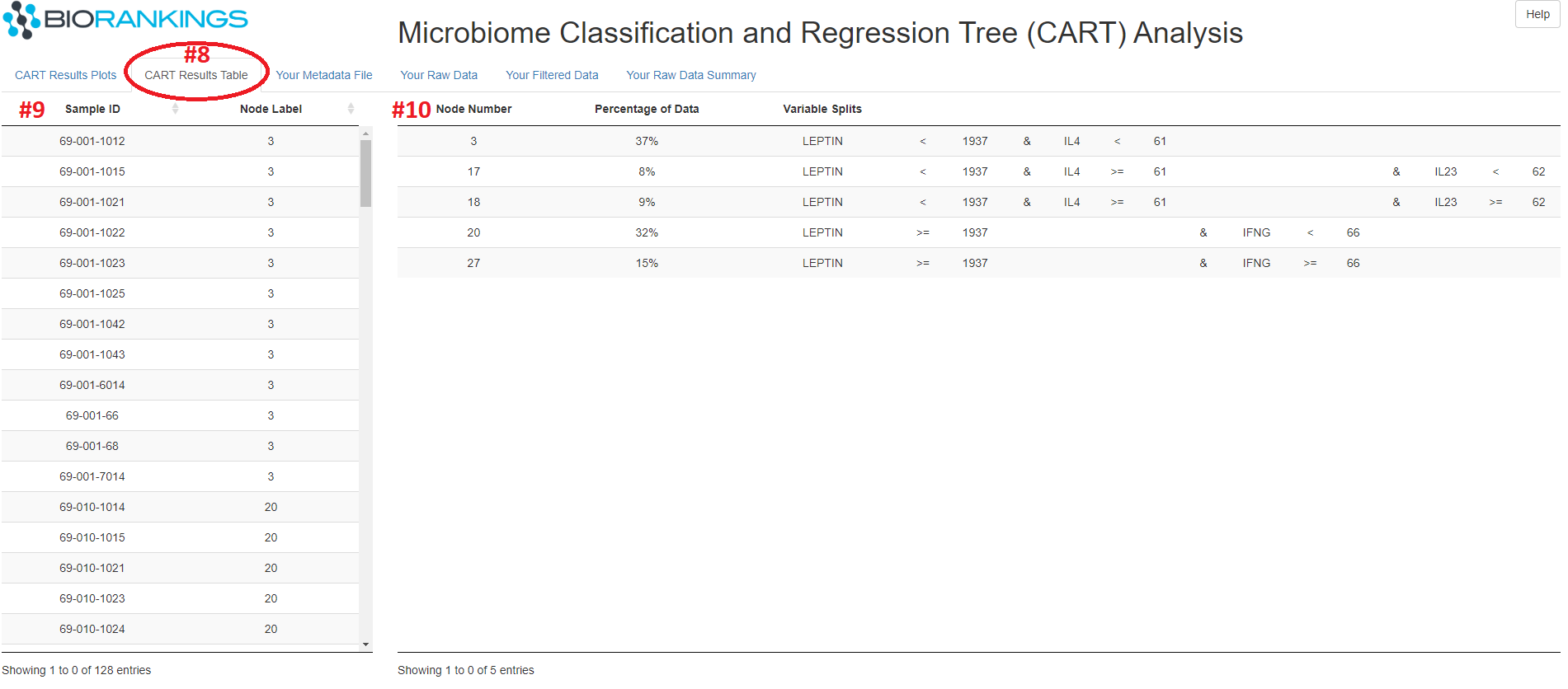
Clicking on the 'CART Results Table' tab (red #8) will bring up the image below. This tab contains
2 tables, the first of which (red #9) shows each samples ID and the terminal node it belongs too.
The second table (red #10) shows a break down of the splitting rules for each terminal node.
For example, the samples in terminal node #3 have a LEPTIN value < 1937 and an IL4 value < 61.
-
The additional tabs display the user entered metadata(red #11), the user entered microbiome count
data (red #12), the filtered microbiome data used to build the tree (red #13) and a summary of the
microbiome data (red #14).

If you have any issues please do not hesistate to contact us